Zero-shot ISP Bandwidth Bands with Timestral

I pointed Mistral’s new time-series model, Timestral 208M, at a month of total bandwidth from a medium-sized ISP’s 100 Gbps network. With no training, no tuning and no calendar features, it produced a threshold band about 45% narrower than the one our product computes today, and it still contained 99.7% of the next day’s actual traffic.

Key points

1. This model is a Zero Shot model because it has never seen actual traffic from this ISP, it has not been trained on it, it is able to forecast only based on the data points in the context window.
2. So small that no GPU is needed.
3. It is a Modified MIT license. I think small companies < $10M revenue can simply bundle this with their software.
4. How far out can it forecast: one pass is 1024 steps. That is about 3.6 days of 5 minute data. But there is no limit, it can continue by feeding its own predictions back and keep going, with potentially diminishing returns.
5. How much history does it need: The context window is 32K steps. That is about 114 days. I just used 1 month or 8K steps. That is about 25% of the window.
6. Blazing fast. 140ms for the 209M model on a CPU only.

Here is what I did, what came out, and a couple of things that tripped me up along the way.

The setup

The data comes from Trisul Network Analytics running on NetFlow from the ISP. Trisul keeps every metric as a time series, and the one I used is the simplest: total bandwidth across the whole network. That’s a single 5-minute series, peaking around 65–70 Gbps in the evening and dropping to about 10 Gbps before dawn.

The plumbing took a few lines:

1. Pull Sep 17 to Oct 14 2026. about 4 weeks of 5-minute data from Trisul over its query API, TRP (protobuf over ZeroMQ). Over a window that long, Trisul returns 5-minute buckets on its own, so there is no resampling.
2. Hand the series to Timestral as one plain array: no timestamps, no weekday or holiday columns, no covariates (holidays or special events).
3. Ask for Oct 15 and Oct 16 2026, the next 288 steps (one day) or 576 steps (two days), and keep the 1% and 99% quantiles as the band.
4. Then check the forecast against what Oct 15 and Oct 16 actually saw. See images below

The code is roughly

from timestral import TimestralForecaster

m = TimestralForecaster.from_pretrained("mistralai/Timestral-209M", device="cpu")
fc = m.forecast(history[None, :], prediction_length=576)   # 2 days of 5-min steps
low, high = fc.quantile(0.01), fc.quantile(0.99)

The 209M model runs on an ordinary laptop CPU and forecasts two days from four weeks of context in well under a second.

Trisul’s existing threshold bands

Trisul already draws a threshold band and raises an alert when traffic leaves it. The method is deliberately simple and has served well for years:

• For each 5-minute slot of the day, take the same slot on the last few same weekdays (5 Thursdays, for next Thursday). So Thursday 10AM to 10:05AM traffic is ONLY ever trained on the last 5 Thursdays 10:00 to 10:05 AM.
• The band is the max and min of those samples.
• At alert time, add a 10% margin and require 5 buckets in a row outside the band before firing.

Timestral gets none of that day-of-week structure. It sees one long series and has to find the daily and weekly rhythm on its own.

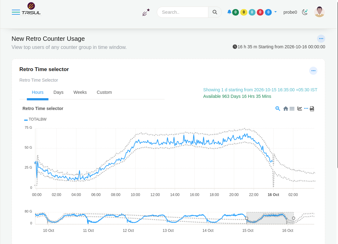
This is what the existing bands look like. The bands are purposely wide to account for the simple algorithm and to prevent spurious alerts. This has been working on several customer networks for a while now.

Timestral forecast much tighter

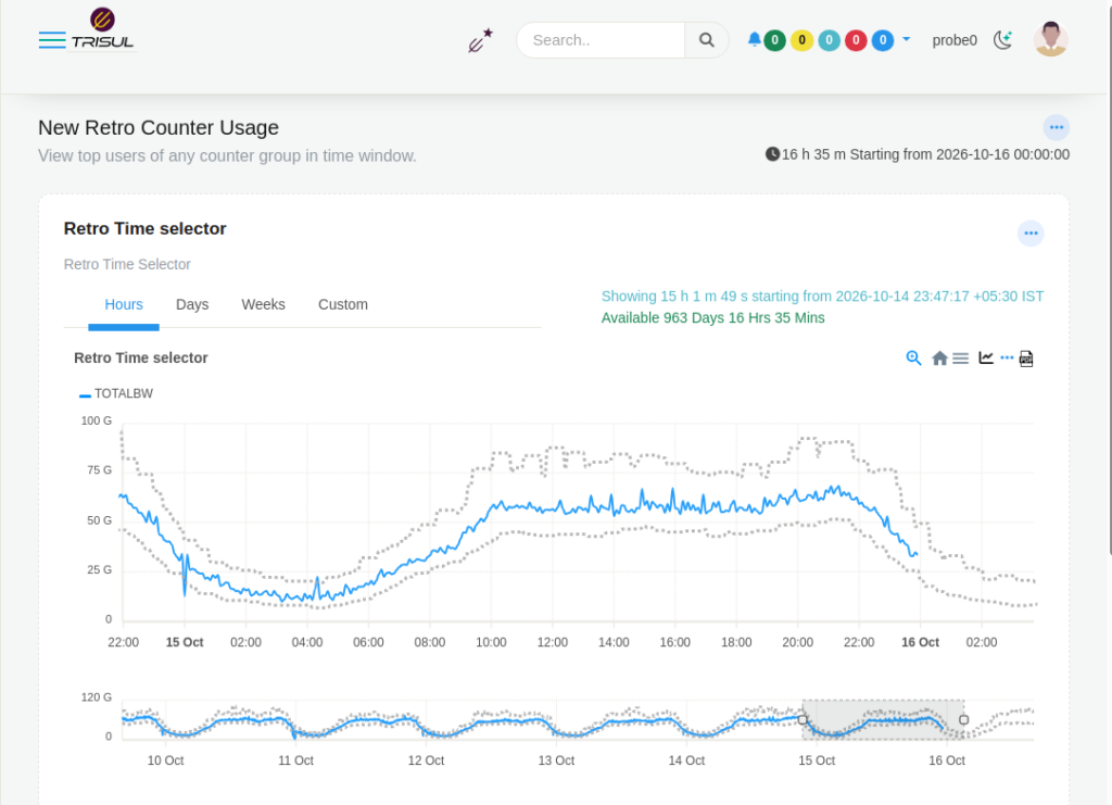
The following picture was Trisul using Timestral to predict the band for Oct 15 2026 and the eventual traffic that was seen. Except for one spike the entire traffic fell into the narrower (45% narrower) range.

How Timestral works is, it does not give one predicted value per 5-min slot. Rather it gives a spread of predictions , 21 numbers to be precise. We use the 99% quantile number for the upper-band and the 1% quantile for the lower-band.

• Say at 10:30 slot
• Upper Band: 99% quantile of 58.5Gbps – means there is only 1% chance the observed value will be greater than this
• Lower Band: 1% quantile of 49.2 Gbps – means there is only 1% change the observed value will be lower than this.

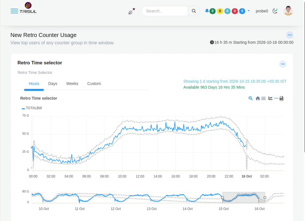
The detail that impressed me most: every night this network’s first bucket after local midnight drops sharply, from about 33 Gbps to about 12 Gbps. This is because this particular ISP resets AAA sessions at midnight, then recovers within 5 minutes. Nobody told the model about it. Its first forecast step after midnight came out at 15.6 Gbps, and every Timestral band I wrote reproduced the dip in the right bucket.

What’s next

We are still catching up with the explosion of directly usable AI technology that isnt just LLMs. We plan to make this forecasting available to number of use cases with labeled co-variates and see how it works in the real world. We also plan to turn on Alerts against a Timestral forecast in production. After that, I want to try it on harder series than the network total: per-application, per-interface and per-customer traffic, also lower bandwidth where the patterns are noisier and a simple envelope struggles more.

Thanks to the Timestral team at Mistral for releasing the model openly and inviting people to try it. Going from download to a working threshold band on real ISP traffic took an afternoon, and most of that was plumbing on our side.

#TimeSeries #Forecasting #NetworkMonitoring #AnomalyDetection #Mistral